Input Parameters

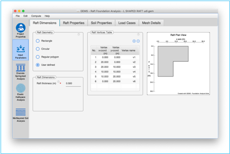
Input parameters pane specifies the dimensions, properties of the raft, soil, and load cases.  These are entered in their respective tabs. 

Raft Dimensions Tab

Raft Dimensions tab defines the raft geometry, coordinates of the raft vertices, thickness of the raft.  It also displays a pictorial view of the raft along with the finite element mesh used for analysis.    

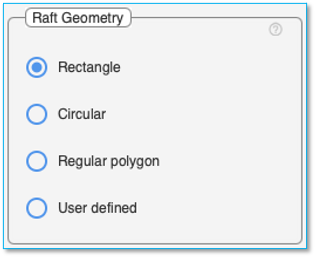
Raft Geometry

Select the raft geometry used for the project in the raft dimensions tab.  The choices for raft geometries are:

a) Rectangular

b) Circular

c) Regular polygon

d) User-defined

Based on the geometry of the raft, define the appropriate parameters of the raft in the adjacent raft dimensions pane.

Table 1 Summary of parameters to be specified for the different raft geometries.

Raft parameter	Rectangular	Circular	Regular polygon	User defined
Raft thickness	✓	✓	✓	✓
Raft length	✓
Raft breadth	✓
Radius of raft		✓
Number of sides			✓
Length of side			✓
Co-ordinates of vertices				✓

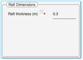
Raft thickness

Specify the thickness of the raft in the units specified.  This field is mandatory and applicable for raft of all geometries.

Rectangular Raft

For rectangular raft define the length and breadth of the raft. Click on [Generate Vertices] button to generate the vertices for the raft. 

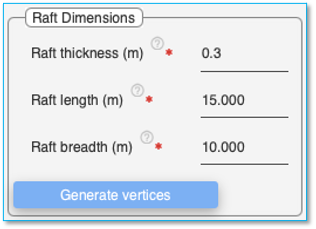
The vertices are shown in the adjacent ‘Raft Vertices Table’. 

Circular Raft

For ‘Circular Raft’ after defining the radius, click on [Generate Vertices] button to generate the vertices for the raft.  The circular raft is approximated as a regular polygonal raft with 12 sides. 

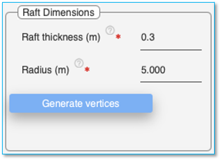
The vertices are shown in the adjacent ‘Raft Vertices Table’. 

Regular Polygon Raft

For ‘Regular Polygon Raft’ after defining the number sides and length of each side, click on [Generate Vertices] button to generate the vertices for the raft. 

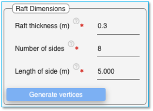
The vertices are shown in the adjacent ‘Raft Vertices Table’. 

User-defined Raft

Define all the vertices in the adjacent raft vertices table.  The vertices need to be defined in sequential order.  If the edges of the raft intersect one another, it will give an error. 

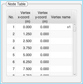
Raft Vertices Table

This table is used to specify the vertices of the raft in sequential order.  The coordinates of the vertices for other geometries are generated in the table when the [Generate Vertices] button is clicked.  The vertices can be named by the user in the ‘Vertex name’ column. 

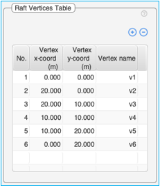
Use the (+) and (-) buttons at the top of the table to add / delete rows to the Raft Vertices Table'. 

Click on the [Generate Mesh] button to generate the finite element mesh.  See ‘Mesh generation’ for additional details.

Table Columns:

Vertex x Coord: Specify the X coordinate of the raft vertex.

Vertex y Coord: Specify the Y coordinate of the raft vertex.

Vertex name: Specify the name of the vertex.  This is optional.

Note: A total of 50 vertices can be specified.

Right click on the table to bring-up the context menu to insert / delete rows in the middle of the table, cut, copy, delete and paste contents into the table.  It is also possible to copy the table from excel and paste the contents into this table.  Ensure adequate number of empty rows are added to the table prior to pasting contents from an excel table.

Mesh Generation

Mesh density

Use the slider to specify the mesh density.  The number of elements in the finite element mesh is roughly proportional to the square of the mesh density selected.  

Use the mesh density to ensure a nicely spaced even mesh is generated. After changing the mesh density, click on the [Generate Mesh] button in the ‘Raft Vertices Table’ to generate the mesh. 

Node points

This field displays the number of node points in the finite element mesh.  A ‘X’ in front of this field indicates that the number of elements exceeds this maximum.  A maximum of 1000 node points is supported for the mesh.  A ‘X’ in front of this field indicates that the number of node points exceeds this maximum.  Adjust the mesh density to arrive at the appropriate mesh.

Elements

This field displays the number of elements in the finite element mesh.  A maximum of 500 elements is supported for the mesh.  A ‘X’ in front of this field indicates that the number of elements exceeds this maximum.  Adjust the mesh density to arrive at the appropriate mesh.

Mesh generation details

The software uses quadrilateral finite element mesh for analysis.  The mesh is generated considering the vertices of the raft, all the concentrated load points across all load cases and the mesh density specified.  For rectangular raft, it tries to fit a rectangular mesh.   For other types of rafts, a mesh consisting of quadrilaterals is generated conforming to the shape of the raft. The mesh nodes include all the load points specified. It is necessary to fill the loads table before generating the mesh.

Raft Diagram

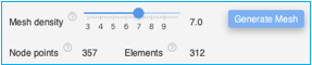
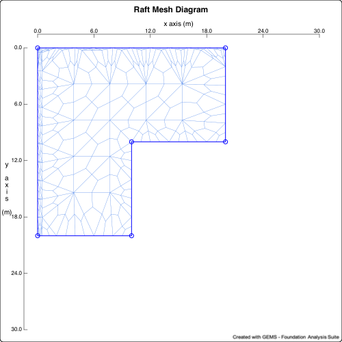
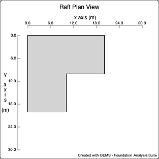
The raft diagram displays the vertices of the raft along with the finite element grid which will be used for computation.

Raft Properties Tab

Raft properties tab is used for specifying the properties of the raft material, self-weight inputs. 

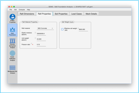
Raft Material Properties

Use the dropdown menu to select the material used for the pile.  The elastic modulus, Poisson ratio of the raft along with the unit weight is updated based on the selection.

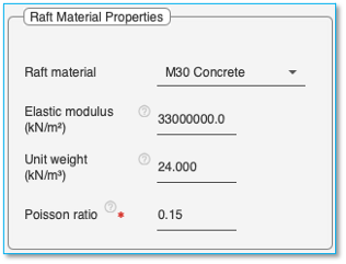
Table 2 Elastic modulus of raft material

Raft Material	Elastic Modulus
	(kN/m^3)	(kips/ft^3)
Steel
ASTMA36	2.0*10^8	4.173 * 10^6
Concrete
M20	3.0 * 10^7	6.26 * 10^5
M25	3.1 * 10^7	6.47 * 10^5
M30	3.3 * 10^7	6.68 * 10^5
M35	3.4 * 10^7	7.10 * 10^5
M40	3.5 * 10^7	7.31 * 10^5
M45	3.6 * 10^7	7.52 * 10^5
M50	3.7 * 10^7	7.73 * 10^5

Select the “User Defined” option to enter values for the elastic modulus and unit weight of the raft material. 

Elastic modulus of raft

The elastic modulus of raft is shown here based on the material specified.  If “User Defined” material is selected, the elastic modulus of the raft can be edited and entered here. 

Poisson ratio of raft

The Poisson ratio of raft is shown here based on the material specified.  The Poisson ratio can be set for all types of raft material.  A default value of 0.15 is used otherwise. 

Unit weight of material

The unit weight of raft material is shown here based on the material specified.  If “User Defined” material is selected, the ‘unit weight of material’ can be edited and entered here.

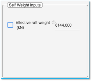
Self-weight inputs

The self-weight properties could be considered for analysis of the raft.  The values of self-weight are auto-calculated based on the raft dimensions or they could be user-defined. 

Effective raft weight

The automatically calculated ‘Effective raft weight’ is shown here as default value. Effective raft weight accounts for the reduction in raft weight due to buoyancy effect of water. The buoyancy effect of water is considered when the depth of water table is specified in the ‘site properties’ section. To enter a user defined value of ‘effective raft weight’, select the checkbox adjacent to this and enter the user defined value in the ‘text field’ next to it.   

Soil Properties Tab

Soil properties tab is used to enter the details of ‘Conventional soil models’ for ‘Discrete Spring-bed analysis’ and ‘Elastic Halfspace analysis’ and soil layers for ‘Multilayered soil analysis’ .   The tab is further subdivided into 2 tabs (on right hand side)

· Conventional Models

· Soil Layers

Soil Properties Tab > Conventional Models Tab

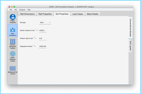
Soil Type – Select the soil type from the drop-down menu.

Parameters for 'Elastic Halfspace Analysis'

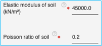
Elastic modulus of soil – Specify the elastic modulus of soil in the text box.  In elastic half-space analysis it is necessary choose the modulus so as to be representative over a depth corresponding of the zone of influence.  

Note on elastic modulus of soil

For clay soil:

The undrained Elastic modulus Eu be preferably obtained from undrained  triaxial compression test on un-disturbed soil samples. The following are some guidance values from literature.

Table 3 Typical Ranges of Eu/Pa values

( Pa = 100 kPa or in 2.12 kips/sq ft.

Clay Consistency	Su (kPa)	Eu/Pa
Soft	< 25	15-40
Medium	25 – 50	40-80
Stiff	> 50	80-200

The following table is compiled from the work of Jamiolkowski et al. as given  in Tomlinson and Woodward

Table 4 Typical ranges of Eu/su

Plasticity index	Over consolidation ratio
	1	2	3	4	10
>50	150 - 300	140 - 280	100 - 250	80 - 210	10-30
30-50	300 - 610	280 - 590	250 - 500	210 - 410	30-150
< 30	610 - 1500	590 - 1420	500 - 1220	410 - 990	150-380

For sand soil: E’

For drained elastic modulus for sand the following correlations with SPT (N60) may be used.

Table 5 Values of E’/Pa for sand (Kulkway and Mayne)

	E’/Pa
Sand with fines	5 x N60
Sand (Normally consolidated)	10 x N60
Sand (Over consolidated)	15 x N60

Table 6 Drained elastic modulus E’/Pa values (Poulos and Davis)

	E’/Pa
Loose sand	100 – 200
Medium dense sand	200 – 500
Dense sand	500 – 1000

Pa = 100 kPa in SI units

Poisson ratio of soil – Specify the Poisson ratio of soil in the text box. 

Note on Poisson ratio of soil

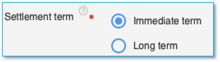
Un-drained elastic modulus coupled with a Poisson ratio value of 0.5 is used for analyzing immediate behaviour. On the other hand, use of drained elastic modulus and drained Poisson ratio are used for analyzing long-term behavior.

Clay (un-drained) ν_u = 0.5

Dense Sand (drained) ν’ = 0.3 - 0.4

Loose sand (drained) ν’ = 0.1 - 0.2

Parameters for 'Discrete Spring-bed analysis'

Subgrade Modulus:

The modulus of subgrade reaction (k1) is usually specified for a plate of size of 1ft x 1ft.   This modulus needs to be modified to account for the following before giving it as data to run the software:

i) Width of foundation

For clay soil

For sandy soil in kips - ft. units

in SI units

ii) Shape Correction:

For rectangle of size mB x B

iii) Depth correction:

This correction is applicable only for granular soil.

Taking all corrections in to account

For clay soils

For granular soils

The values of subgrade modulus entered as data should incorporate all corrections.

In the absence of field or laboratory data the following values proposed by Terzaghi may be used.

Values of modulus of subgrade reaction k1 for 1ft x 1ft square plates in kips/ft³

Granular Soil

Relative Density	Low	Medium	Dense
Dry or moist sand - limiting values	40-120	120-600	600-2000
Proposed values for dry moist sand	80	260	1000
Proposed values for submerged sand	50	160	600

Values of modulus of subgrade reaction k1 for 1ft x 1ft square plates in kips/ft³

Clay Soil

Consistency	Stiff	Very stiff	Hard
Unconfined compressive strength(ksf)	2-4	4-8	> 8
Range of values	100-200	200-400	> 400
Proposed values for submerged sand	150	300	600

Values of modulus of subgrade reaction k1 for 1ft x 1ft square plates in kN/m³

Granular soil

Relative Density	Low	Medium	Dense
Dry or moist sand - limiting values	6300-18900	18850-94250	94250-157100
Proposed values for dry moist sand	12570	40850	157100
Proposed values for submerged sand	7850	25130	94250

Values of modulus of subgrade reaction k1 for 1ft x 1ft square plates in kN/m³

Clay soil

Consistency	Stiff	Very stiff	Hard
Unconfined compressive strength(kPa)	50-100	200-400	>400
Range of values	15710-31420	31420-62840	>62840
Proposed values for submerged sand	23560	47120	94250

Soil Properties Tab > Soil Layers Tab

Soil Properties Tab is used to enter the data about the site condition, sub-soil layers and properties of each soil layer.  It is divided into 3 panes

· Site Condition

· Soil Layer Table

· Soil Layer Properties

This tab is mandatory for ‘Multilayered soil analysis’.

Soil Properties Tab > Soil Layers Tab > Site Condition

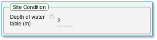
Depth of water table

This field is not mandatory. Specify the depth of water table at the site in the field provided. 

If no value is specified, it is assumed the water table lies below all the layers of soil specified.  For water table at ground level, set it as 0. 

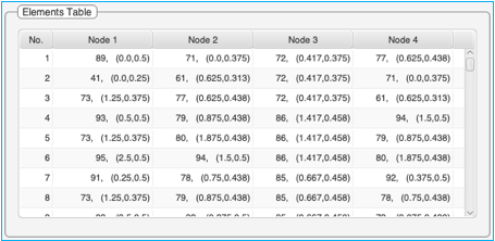
Soil Properties Tab > Soil Layers Tab > Soil Layer Table

The ‘Soil Layer Table’ is used to define the type of soil and the thickness of each layer of soil. The properties of the soil layer selected is entered in the adjacent ‘Soil Layer Properties’ pane. 

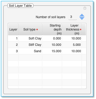
Number of soil layers

First select the number of soil layers using the up/down arrow.  This will set the number of rows in the table to populate

Up 20 soil layers can be specified.

Note: For TRIAL version, number of soil layers is restricted to 3.

Table: Double-click on the table cells to edit the content of the cells.

The table consists of four columns – Layer, Soil type, Starting depth and Layer thickness.  The ‘Layer’ column and the ‘Starting depth’ columns cannot be edited. 

To enter the Soil type, click on the cell in this column and select the type of soil from the ‘drop down’ menu for each segment.

Permissible soil types currently are – Soft Clay, Stiff Clay, Sand, Weak Rock, and Hard Rock.    

You can use ‘Sand’ to represent silt, silty sand, and gravel as well.

Layer thickness Column – This defines the thickness of each layer of soil.

Starting depth Column – This column is auto calculated based on the thickness of soil layers entered. 

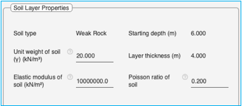
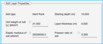
Soil Properties Tab > Soil Layers Tab > Soil Layer Properties

Select a layer in the ‘Soil layer table’ to display the soil properties associated with it in this pane. 

Note: Mandatory fields have a () adjacent to them depending on the choices made for capacity estimation, axial pile analysis and lateral pile analysis.

Note: The soil layer properties need to be arrived at from the soil investigation report.  The application populates median recommended values for each property.  These values need to be updated with actual values from the soil investigation report or values chosen by the user.

Common properties for all soil types:

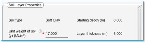
Soil type: Shows the type of soil in this layer.  (Field cannot be edited)

Unit weight of soil (γ): The unit weight to be given as data is the total unit weight of soil in the layer that is the moist unit weight above the water table and saturated unit weight below the water table. If required one may choose to divide the layer in to two halves one above water table and the other below the water table having different unit weights.

Starting depth: Displays the starting depth of the layer. (Field cannot be edited)

Layer thickness: Displays the thickness of the selected layer.  (Field cannot be edited)

Properties for Soft Clay soil

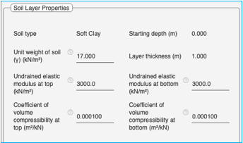
Table 7 Soil property details for soft clay soil

Soil property	Units	Min value	Max value	Notes
Undrained elastic modulus	kN/m^2	1750	5000	Value of 0 is only permissible for the top of the first soil layer. Required for immediate term behaviour.
	kips/ft^2	36.54	104.4
Coefficient of volume compressibility (mv)	m^2/kN	4 * 10^-4	10^-3	Required for long term behaviour.
	ft^2/kips	1.91 * 10^-2	4.78 * 10^-2

Please see the note on Elastic modulus and Poisson ratio

Note on coefficient of volume compressibility (mv)

The Coefficient of volume compressibility (mv) should be chosen from the laboratory consolidation test results on undisturbed soil sample. The e-logp curve should be corrected in the case of pre-loaded clay.  The coefficient of volume compressibility may be directly read from the e-p curve as

Or from the e-logp curve as

Where

 = compression index

 =In-situ void ratio

  = vertical effective stress

Properties for Stiff Clay soil

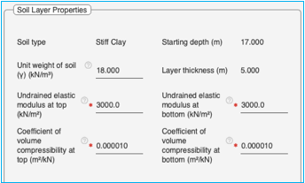
Table 8 Soil property details for stiff clay soil

Soil property	Units	Min value	Max value	Notes
Undrained elastic modulus	kN/m^2	4000	20000	Value of 0 is only permissible for the top of the first soil layer. Required for immediate term behaviour.
	kips/ft^2	83.5	208.8
Coefficient of volume compressibility	m^2/kN	2 * 10^-5	2.5 * 10^-4	Required for long term behaviour.
	ft^2/kips	9.57 * 10^-4	1.19 * 10^-2

Please see the note on Elastic modulus and Poisson ratio for additional details

Please see the note on Coefficient of volume compressibility for additional details.

Properties for Sand soil

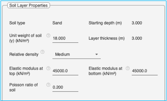
Relative density:  Select the relative density of the sand soil from the dropdown menu.  The choices are ‘Very Loose’, ‘Loose’, ‘Medium’, ‘Dense’ and ‘Very Dense’ sand. 

Table 9 Soil property details for sand

Soil property	Units	Min value	Max value	Notes
Elastic modulus	kN/m^2	11000	200000	Value of 0 is only permissible for the first soil layer at the top.
	kips/ft^2	229.68	4176
Poisson Ratio		0.1	0.5	Default value: 0.2

Please see the note on Elastic modulus and Poisson ratio for additional details.

Properties for Weak Rock

Table 10 Soil property details for weak rock

Property	Units	Min value	Max value	Notes
Elastic modulus of soil	kN/m^2	10^6	2*10^7
	kips/ft^2	20880	417600
Poisson Ratio		0.1	0.5	Default value: 0.2

Properties for Hard rock

Table 11 Property details for hard rock

Rock Property	Units	Min value	Max value	Notes
Elastic modulus of soil	kN/m^2	1.5*10^7	10^8
	kips/ft^2	313200	2088000
Poisson Ratio		0.1	0.5	Default value: 0.25

Load Cases Tab

The ‘Load Cases’ tab is used to enter details of the loading on the raft.

It is important to first specify the ‘Number of load-cases’ in the ‘Project Properties Pane’.  This will setup the appropriate number of tabs under the ‘Load Cases Tab’ for specifying the details of each load case. 

Each load-case should be entered in a separate tab (on the right-hand side).  Each load case tab consists of details of the load applied on the raft along with a loading diagram that graphically represents the same.

Load Case Description

Enter the description of the load case for your reference.  This is an editable text field. 

Include ‘self-weight’ in analysis

Select this checkbox if the weight of the raft is to be included in the analysis. 

The “self-weight” of the raft from the ‘Self weight inputs’ pane in the ‘Raft Properties’ tab is used. 

Settlement term

For multi-layered soil analysis, immediate settlement or long-term settlement can be determined.  Select the appropriate settlement timeline.

Uniform Load

Specify the uniform load applied on the entire raft. 

Concentrated Load Table

This table is used to specify the concentrated loads and moments applied on the raft. 

Use the (+) and (-) buttons at the top of the table to add / delete rows to the ‘Concentrated Load Table'. 

[Organize] button can be used to clean up empty entries in the table. 

Table Columns:

x coord: Specify the X coordinate where the load is applied.

y coord: Specify the Y coordinate where the load is applied.

Fz: Specify the vertical load applied at the point.  Compressive loads (+ve) values act downward while tensile loads (-ve) values act upwards. 

Mx: Specify the moment along the X direction applied at the point. 

My: Specify the moment along the Y direction applied at the point. 

Note: A total of 100 concentrated loads can be applied on the raft

Right click on the table to bring-up the context menu to insert / delete rows in the middle of the table, cut, copy, delete and paste contents into the table.  It is also possible to copy the table from excel and paste the contents into this table.  Ensure adequate number of empty rows are added to the table prior to pasting contents from an excel table.

Loading Diagram

The loading diagram represents the vertical load, moments applied on the raft for a load case.

Bibliography

Bowles, J E. Foundation analysis and Design. Fifth Edition. McGraw Hill, 1996.

Cook, R. D. Concepts and application of finite element analysis. 2nd. McGraw Hill, 1981.

Fleming, K, et al. Piling Engineering. Third. London: Taylor & Francis, 2009.

Harr, M. E. Foundation of theoretical soil mechanics. McGraw Hill, 1966.

Krishnamoorthy, C. S. Finite element analysis - Theory and programming. Tata McGraw-Hill, 1995.

Kulkway, F. H. and P. W. Mayne. Manual on estimating soil properties for foundation design. Ithaca, NY: Cornell University, 1990.

Peck, R. B., W. E. Hanson and T. H. Thornburn. Foundation Engineering. New York: Wiley, 1974.

Poulos, H. G. and E. H. Davis. Pile Foundation Analysis and Design. 1980, n.d.

Terzaghi, K. “Estimation of coefficient of subgrade reaction.” Geotechnique Vol.5.No. 4 (1955): 41-50.

Terzaghi, K., R. B. Peck and G. Mesri. Soil Mechanics in Engineering Practice. Third Edition. New York: John Wiley, n.d.

Timoshenko, S. and Woinowsky-Krieger. Theory of plates and shells. 2nd. McGraw Hill, 1959.

Tomlinson, M. and J. Woodward. Pile Design and Construction Practice. Fifth Edition. London: Taylor and Francis, n.d.